Volumetric fields

v_ase keeps scalar grids in the Python backend and sends only compact metadata, isosurface meshes, and sampled planar rasters to the browser. This allows large DFT fields to remain aligned with their ASE structure without serializing the complete 3D array into the page or an AI-agent context.

Supported inputs 

Open these directly or add them to an existing document:

VASP CHG/CHGCAR charge density;
VASP PARCHG partial density;
VASP LOCPOT potential;
VASP ELFCAR electron-localization field;
Gaussian Cube; and
XSF DATAGRID_3D, including Quantum ESPRESSO pp.x exports.

VASP stems accept ., _, or - calculation suffixes, including PARCHG_band_12, LOCPOT.vacuum, and CHGCAR-difference. Use an explicit reader for an ambiguous filename:

v_ase gui GRID --format CHGCAR
v_ase gui charge.dat --format qe-cube
v_ase gui potential.dat --format qe-xsf

Opening a volumetric file creates the associated atomic structure and one or more scalar dataset descriptors. In an existing document, use Analysis > Volumetric Data > Add Grid Data.

Choose precision before import 

Import precision and the CLI option select storage precision while reading:

v_ase gui CHGCAR --volumetric-precision fp32
v_ase gui CHGCAR --volumetric-precision fp64

Python exposes the same choice:

from v_ase.visualize import view

view("CHGCAR", volumetric_precision="fp64")

FP32 is the lower-memory default.
FP64 preserves double-precision input and uses twice the grid memory.

Changing a display control later does not convert the stored dataset. Verify the descriptor’s precision and backend memory size after loading.

Dataset state 

Each dataset has a stable ID and reports scientific metadata including:

source name and canonical format;
quantity, component, units, and precision;
grid dimensions, cell, origin, and PBC;
endpoint convention and memory bytes;
minimum, maximum, mean, and integral; and
fixed 256-bin raw and absolute-value histograms.

Histogram counts sum to the source voxel count and remain unchanged when isosurface, plane, camera, color, or opacity settings change. Select datasets by ID rather than list position when automating a multi-grid document.

Interpret the integral

VASP charge grids are divided by cell volume on import; their integral equals the average raw grid value (the electron count for an ordinary total-charge grid). LOCPOT values retain eV and are not divided by volume. Cube and XSF retain their reported/native scalar units; do not infer an electron count from an unlabeled field.

Endpoint-exclusive grids use equal voxel weights. For endpoint-inclusive grids, periodic closing planes are excluded once, while finite axes use trapezoidal half weights at both endpoints. The determinant of the complete triclinic cell supplies the volume Jacobian. mean is the arithmetic mean of stored samples; it need not equal the integration-weighted mean on an endpoint-inclusive grid.

Source grids are immutable analysis inputs

Isovalue changes, Gaussian smearing, mesh smoothing, color, opacity, and planar sampling operate on display products. They do not replace the stored FP32/FP64 scalar field, its integral, or the arrays used in a linear combination.

Create an isosurface 

Open Analysis > Volumetric Data > Isosurface:

Select a Dataset.
Enable Show isosurface.
Choose Single level or Positive + negative.
Set a finite Isovalue.
Choose mesh detail, colors, opacity, smearing, and smoothing.
Select Update Isosurface.
Inspect the rendered topology from more than one camera direction.

A newly loaded nonconstant dataset is selected and displayed at an in-range default level. Replace that preview value with the scientifically requested threshold before publishing a result.

Signed volumetric isosurfaces

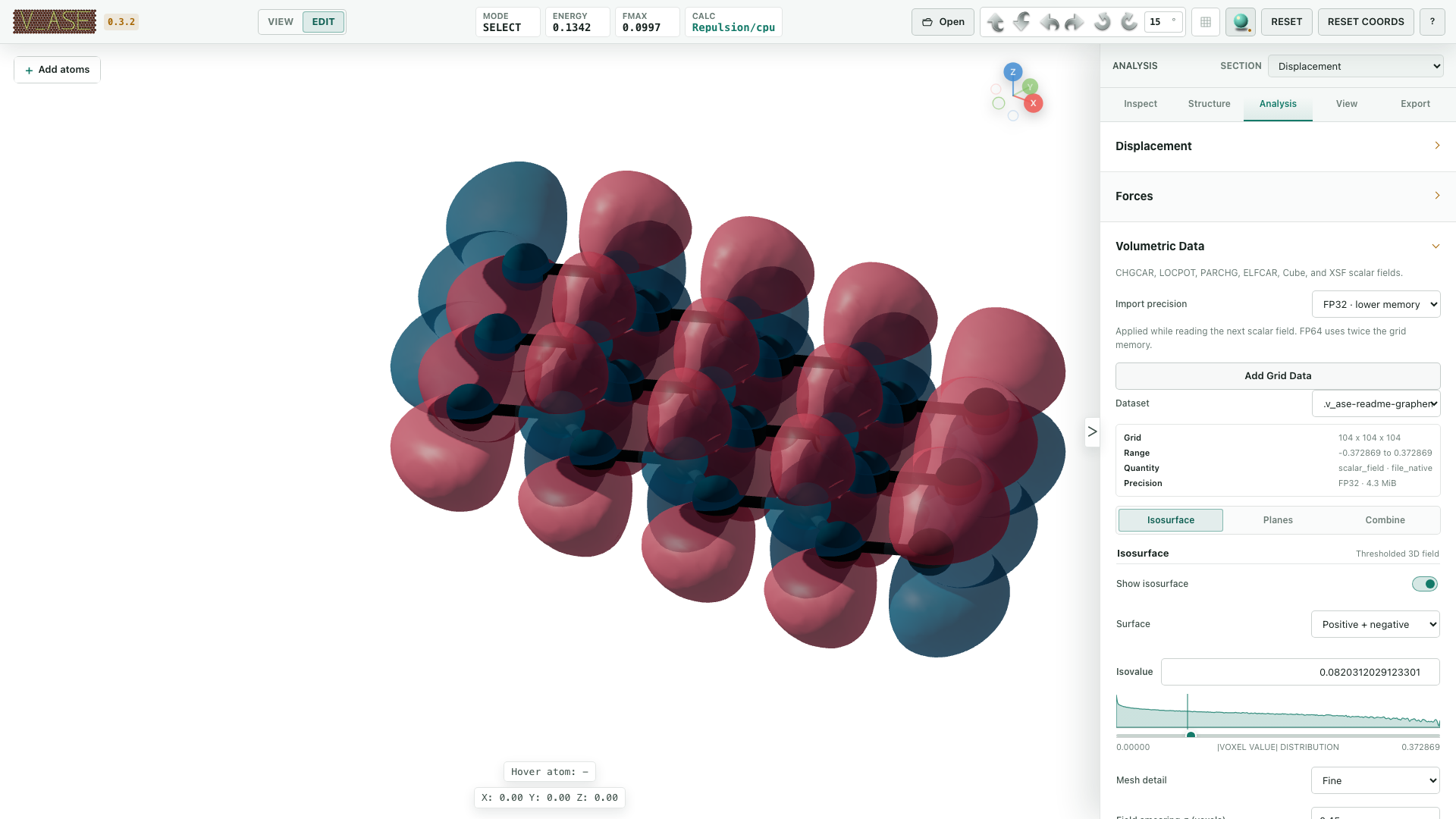
Single and signed levels

Single level requests one finite scalar level. Positive + negative uses the magnitude of a nonzero level and extracts +abs(level) and -abs(level) with independent colors.

After field smearing, one requested sign may lie outside the displayed range. v_ase retains the valid sign, marks the result as a partial signed surface, and does not invent the missing mesh. Verify rendered levels and surface count.

Mesh detail

The semantic mesh step is 1, 2, or 4:

1 / Fine preserves the most grid detail;
2 / Balanced reduces work; and
4 / Fast is the coarsest preview.

Use the smallest step needed to preserve the features of interest. Repeating the same dataset, level, sign mode, detail, smearing, and smoothing request reuses a bounded mesh cache. Changing only color or opacity restyles the existing browser mesh without rerunning marching cubes.

Field smearing

Field smearing σ (voxels) accepts 0 through 8. It applies a Gaussian filter to a display copy before surface extraction. Periodic axes wrap and nonperiodic axes reflect at their boundaries.

Sigma is measured in grid steps, so equal sigma on differently spaced or skew axes is not an isotropic Gaussian in physical Å. Use it as a display filter.

Smearing can merge small features or move an isovalue outside the displayed range. Start around 0.3–0.5 only when grid artifacts require it, compare against 0, and do not describe a heavily smeared topology as raw data.

Mesh smoothing

Mesh smoothing passes accepts integer 0 through 30. It fairs the extracted mesh after marching cubes while fixing cell-boundary vertices. It does not smooth the source field. Use 0 to disable it.

Colors and opacity

Positive/negative colors are six-digit hexadecimal colors. Isosurface opacity is 0.05–1. These are presentation settings and do not affect scalar values. Isosurfaces follow display replication and visual translation with the atoms.

Inspect the result scientifically 

The active surface summary reports:

dataset ID and source range;
requested and rendered levels;
post-smearing display minimum and maximum;
smearing sigma and smoothing passes;
surface and triangle counts; and
whether a signed surface is partial.

An HTTP success is not enough. Render the result, check that it is nonblank, inspect cell seams and topology, then compare the source dataset descriptor to confirm the display refinement did not replace it.

Add planar sections 

Open Analysis > Volumetric Data > Planes and choose Add Plane. Each plane contains:

stable ID and editable name;
dataset ID and visibility;
a nonzero reciprocal-space (h k l) normal;
signed distance from the stored grid origin in angstrom;
settled resolution of 128, 256, 512, or 1024;
a registered Matplotlib colormap and reverse state;
automatic or manual vmin/vmax; and
opacity.

(h k l) defines a Cartesian normal using the reciprocal cell. [0,0,0] is invalid. The distance is measured from the dataset’s stored grid origin along that unit normal, not from an atom, selection, or inferred cell center. If no offset is supplied, v_ase centers the plane in the displayed cell/supercell.

The backend clips the section to the exact orthogonal or triclinic displayed cell and samples it with periodic trilinear interpolation. Only the compact 2D raster and clipping polygon reach the browser; displayed supercells do not materialize a repeated 3D grid.

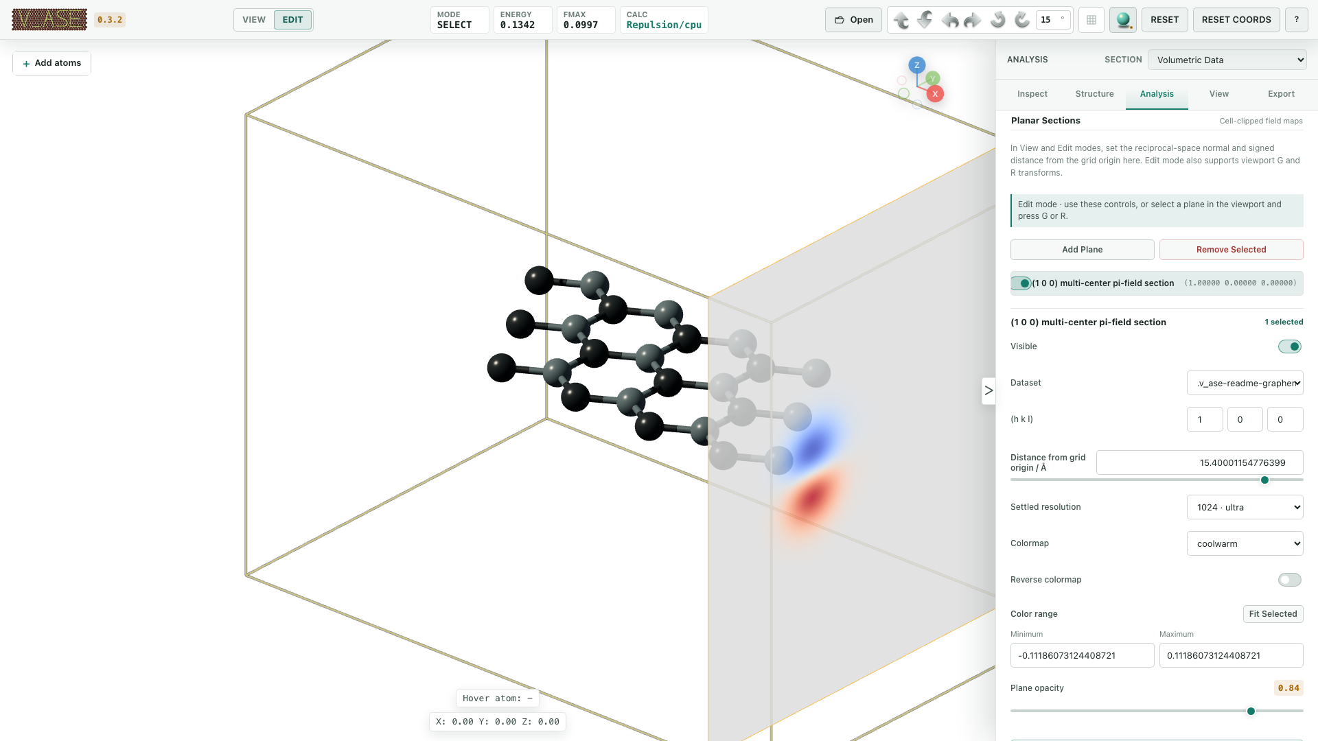
Cell-clipped hkl scalar-field plane

Edit one or several planes

Select plane rows with click or Shift-click. Shared values remain visible; mixed values are blank until a common replacement is entered. One edit is applied atomically to every selected ID. An unknown ID, zero normal, unsupported resolution/colormap, opacity outside its range, or manual vmin >= vmax rejects the complete edit.

Use Fit Selected to resolve the range from the selected plane data. Use a fixed manual range when several planes must remain directly comparable.

View and Edit mode behavior

Planes can be created and configured in View. This changes only analysis and display state, never ASE atom coordinates.

In Edit, a selected plane can also be manipulated in the viewport:

G moves each selected plane along its own normal; and
R, optionally locked with X, Y, or Z, changes the normal and (hkl).

The distance, slider, (hkl) fields, and list label follow the live transform. Interactive motion uses a lower-resolution preview, then restores the configured settled resolution. A newly typed (hkl) becomes authoritative immediately even if an older high-resolution request is still pending.

Combine compatible datasets 

Combination accumulates bounded slabs in FP64 and rounds once to the requested output precision. FP32 remains the memory-saving default when all inputs are FP32; import FP64 before subtraction when small differences matter. Converting an already rounded FP32 source later cannot recover lost input digits.

Open Analysis > Volumetric Data > Combine and enter finite coefficients. A common charge-density-difference form is:

Δρ = ρ_combined - ρ_fragment_A - ρ_fragment_B

The source datasets must match exactly in:

grid dimensions;
cell and origin;
PBC and endpoint convention; and
physical units.

v_ase refuses mismatched grids instead of silently interpolating or resampling. When output precision is omitted, a combination promotes to FP64 if any input is FP64; otherwise it remains FP32. The new dataset receives its own stable ID, descriptor, and histogram.

Cell, replication, and reset behavior 

Visual display.supercell repeats the isosurface and planes with the atoms without changing stored data. Visual translation moves atoms, bonds, constraints, surfaces, and planes together.

Set Supercell as Cell physically repeats atoms and every stored volumetric grid for a diagonal integer repetition, with one atomic Undo entry. A general non-diagonal cell matrix is rejected while grids are loaded because an explicit scientific interpolation policy would be required.

After a materialized diagonal supercell, RESET COORDS restores the original atoms, cell, and scalar grids together. Undo/Redo preserves the atom/grid pairing.

Save and export volumetric work 

Reopening a project restores and samples all visible saved planes before the document reports ready, so its first render includes the same planar rasters.

A .vase project retains stored datasets, precision, current frame, visual settings, and supported analysis state without pickle. A project-embedded HTML save contains the complete validated .vase plus a browser-ready view. Lightweight HTML contains the rendered/view-only scene but is not a lossless editable scalar-grid interchange.

Images and HTML use the persistent Render Area. Before export, verify surface or plane visibility, opacity, crop, camera, axes, cell, background, and exact render dimensions. Use .vase as the editable source of truth.

Semantic workflow 

These are separate JSON request bodies for v_ase api ... apply --params-file. They are not a single script. Fetch the current revision and dataset/plane IDs with describe; the numbers and IDs below illustrate the fields to replace.

Load a field

Load a grid from a path confined to the directory in which v_ase gui was launched:

{
  "expectedRevision": 12,
  "operation": {
    "name": "load-volumetric",
    "path": "charge/CHGCAR",
    "precision": "fp64"
  }
}

Display a signed surface

Call describe, take the returned stable dataset ID, then create an exact surface:

{
  "expectedRevision": 13,
  "operation": {
    "name": "show-volumetric",
    "datasetId": "DATASET_ID",
    "level": 0.015,
    "surfaceMode": "signed",
    "stepSize": 1,
    "smearingSigma": 0.4,
    "smoothingIterations": 6,
    "opacity": 0.72,
    "positiveColor": "#2a9d8f",
    "negativeColor": "#d1495b"
  }
}

Add a crystallographic plane

Add a plane:

{
  "expectedRevision": 14,
  "operation": {
    "name": "add-volumetric-plane",
    "datasetId": "DATASET_ID",
    "planeName": "(1 1 0) section",
    "hkl": [1, 1, 0],
    "offsetAngstrom": 2.5,
    "resolution": 512,
    "colormap": "viridis",
    "reverse": false,
    "autoRange": true,
    "opacity": 0.9,
    "visible": true
  }
}

Change plane colors and range

Edit or remove planes only with IDs returned by describe().analysis.volumetricPlanes:

{
  "expectedRevision": 15,
  "operation": {
    "name": "update-volumetric-planes",
    "planeIds": ["PLANE_A", "PLANE_B"],
    "colormap": "coolwarm",
    "autoRange": false,
    "vmin": -0.08,
    "vmax": 0.08,
    "opacity": 0.82
  }
}

Subtract fragment fields

Combine fields. name selects the command and resultName labels the output:

{
  "expectedRevision": 16,
  "operation": {
    "name": "combine-volumetric",
    "datasetIds": ["COMBINED", "FRAGMENT_A", "FRAGMENT_B"],
    "coefficients": [1, -1, -1],
    "resultName": "charge-density difference",
    "precision": "fp64"
  }
}

Related operations are load-volumetric, show-volumetric, add-volumetric-plane, update-volumetric-planes, remove-volumetric-planes, combine-volumetric, and remove-volumetric. Use the current collaboration revision on every mutation. The numeric revisions in these examples are illustrative; describe is the source of the next exact value.

Limits and failure behavior 

A scalar array must be three-dimensional with at least two samples per axis.
The default source-grid ceiling is 134,217,728 points. Override V_ASE_MAX_VOLUMETRIC_POINTS only after confirming available memory.
The default surface safety ceiling is 2,000,000 triangles per surface.
Smearing is limited to 0–8 voxels; smoothing to 0–30 passes.
Semantic surface step is 1, 2, or 4; plane resolution is 128, 256, 512, or 1024.
Dataset removal requires an exact stable ID.
Relative semantic paths cannot escape the GUI launch directory.
Constant fields remain stored but cannot produce an isosurface crossing.
A mismatched linear combination or invalid plane edit is rejected without partially mutating the document.

Verification checklist 

Before presenting a volumetric result, record and verify:

source filename/type, quantity, component, units, precision, and memory;
grid dimensions, cell, origin, PBC, and endpoint convention;
raw minimum/maximum/integral and histogram mode;
dataset ID, isovalue, sign mode, detail, smearing, smoothing, opacity, and rendered mesh counts;
for every plane: ID, nonzero (hkl), signed offset, resolution, map, range, opacity, visibility, and displayed-cell repetition;
exact compatibility and coefficients for a linear combination;
atom/grid alignment after translation, replication, frame change, Undo, or reset; and
a decoded, nonblank render inspected from the intended camera.