Trajectories and analysis

v_ase keeps the displayed trajectory frame, atom identities, stored properties, vectors, volumetric assignments, and plotted analyses synchronized. This page covers source and optimizer timelines, displacement, stored forces, per-atom property coloring, and radial or finite pair distributions.

Open a trajectory

v_ase gui trajectory.extxyz
v_ase gui XDATCAR --index :
v_ase gui relaxation.traj --index -1
v_ase gui dump.lammpstrj --stream-frames

--index : selects all frames, -1 selects the last frame, and an integer selects one zero-based frame. A loaded file starts in View unless --interactive is supplied.

Lazy and streamed sources

View mode can avoid materializing the whole trajectory:

• XDATCAR uses coordinate byte offsets when its layout can be proved safe;

• native ASE .traj uses random access;

• compatible numeric LAMMPS dumps use a byte-indexed, memory-mapped path; and

• --stream-frames requests frames individually for other supported local sources.

Remote HOST:/path inputs always keep frame storage and parsing on the remote host. Switching to Edit materializes the frames required for topology-wide physical operations. An unsupported fast layout falls back to the compatible ASE reader instead of guessing.

Timeline controls

Use the bottom timeline or keyboard:

Control	Action
Space	Play or pause the active timeline
Left/Right Arrow	Previous or next active-timeline frame
Previous/Next buttons	Step one frame
FPS	Playback rate
Skip	Advance by more than one source frame

v_ase can show several timeline kinds without merging them:

• Source frames loaded from a file or Python sequence;

• ordinary structure Relaxation frames;

• Add Atoms placement-relaxation frames; and

• Rigid Translation registry-relaxation frames.

The selected timeline alone receives playback and arrow-key input. Optimizer timelines are mode state, not silently appended source trajectories.

Add or replace frames

Open can replace the current document, append compatible frames, or open a new tab. Appending keeps the active frame, camera, and visual state. Appending a .vase imports only its structures; replacing or opening it in a new tab restores the complete saved project.

If appended frames introduce new labels, v_ase registers them without discarding existing appearance. A variable atom count or changed element order is allowed for inspection but limits identity propagation and some analysis.

Frame identity and selection

Selection persists by stable atom index when topology permits. For a stable atom count and element order, View-mode visual labels and atom-index appearance can follow the same particles through the trajectory. If topology is incompatible, v_ase exposes the mismatch and limits changes to valid frames instead of applying an incorrect identity globally.

Do not reuse an atom index merely because the viewport looks similar. Verify the active frame, count, labels, chemical elements, and any particle-ID array before a coordinate-dependent operation.

Ordered geometry through a trajectory

Select atoms in the intended order:

• one atom shows label, element, displayed Cartesian/fractional position, and lazy per-atom properties;

• two show direct and minimum-image distances where applicable;

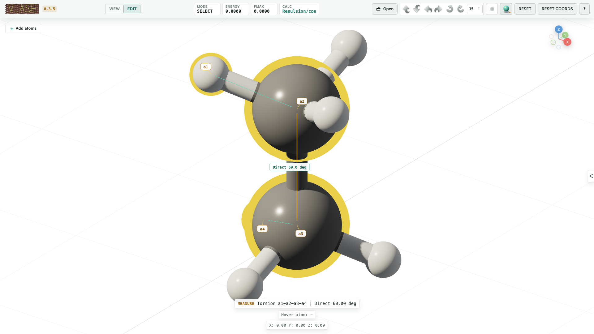
• three show the a1-a2-a3 angle at a2;

• four show the signed a1-a2-a3-a4 torsion; and

• larger selections show total and per-label counts.

The retained Measure overlay follows the selected source or optimizer frame and committed G/R/S edits without relying on hover state.

Displacement analysis

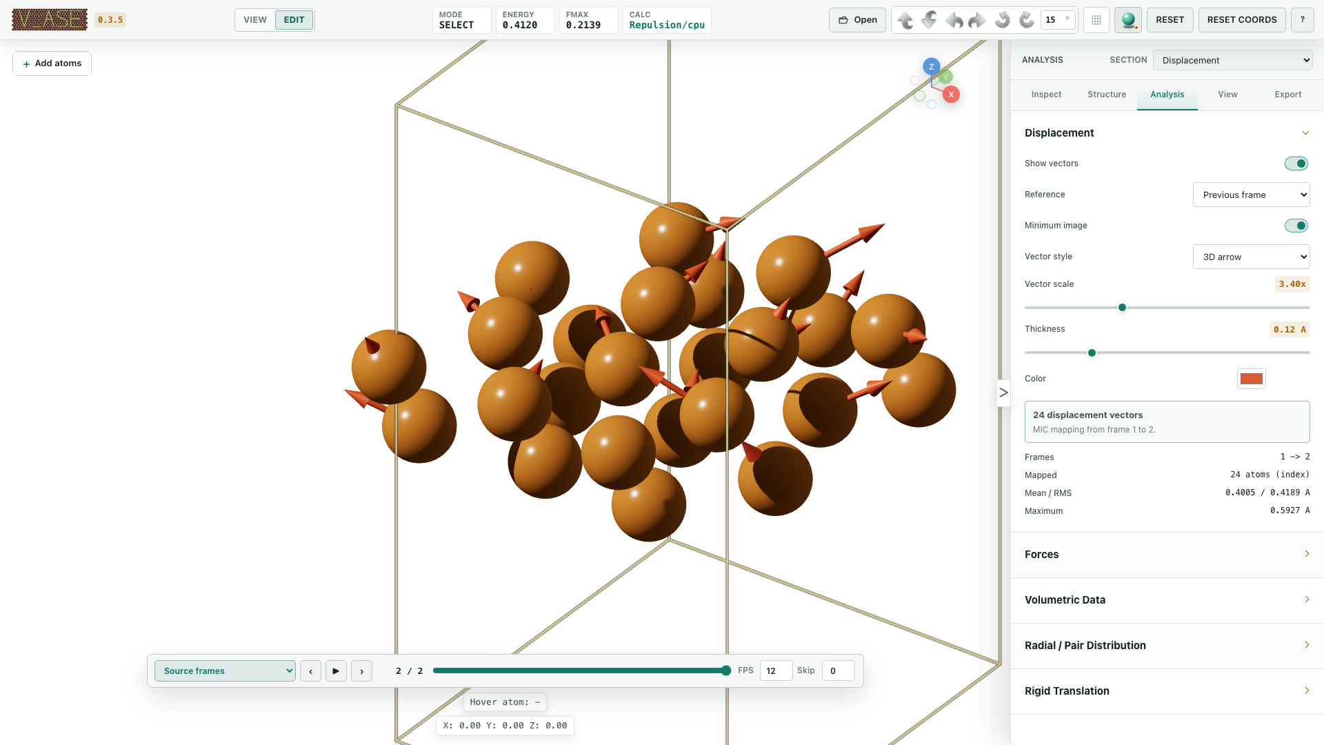
Open Analysis > Displacement and enable Show vectors.

1. Choose Previous frame or Specific frame as reference.

2. For a specific reference, enter its displayed one-based frame number in the GUI.

3. Keep Minimum image enabled for periodic particle motion unless an unwrapped Cartesian path is intentionally required.

4. Choose 3D arrow or 2D flat arrow.

5. Adjust vector scale, thickness, and color.

The backend prefers a common unique particle-ID array. Equal-size frames can fall back to atom index. Different-size frames without a valid mapping return an error rather than pairing unrelated atoms.

Displacement vectors retain physical values. The renderer anchors them at current visible positions, repeats them with displayed supercells, and applies the same visual translation to both endpoints. Scaling changes arrow length, not the stored displacement.

Stored force vectors

Stored SinglePointCalculator forces are retained when frames are copied for analysis. Semantic structure/full descriptions read the displayed frame’s exact stored properties even when force arrows are hidden; compact descriptions return property counts, and includeProperties:true requests the arrays.

Open Analysis > Forces and enable Show vectors. Choose 3D/2D style, length scale, thickness, and color.

Force arrows use only values already stored on the active frame in an ASE array or calculator result. v_ase does not run an attached calculator merely to draw an arrow. If forces are missing or nonfinite, the feature remains unavailable rather than reusing another frame’s buffer.

For stored Cartesian vector F, the displayed direction is exactly the direction of F and the arrow length is:

forceVectorScale × |F|

Displayed supercells repeat arrows with their atoms. During playback, force vectors and scalar colors are reloaded from the same active frame.

Inspect one atom’s stored properties

One selected atom exposes properties lazily for the active frame. The detail can include:

• index, symbol, label, position, mass, tag, charge, and magnetic moment;

• arbitrary scalar, string, vector, or tensor entries from Atoms.arrays;

• stored calculator results; and

• stored Cartesian forces.

The property request never evaluates a calculator. A selected replica uses the base atom’s property payload while retaining its displayed replica position for measurement.

Map numeric per-atom data

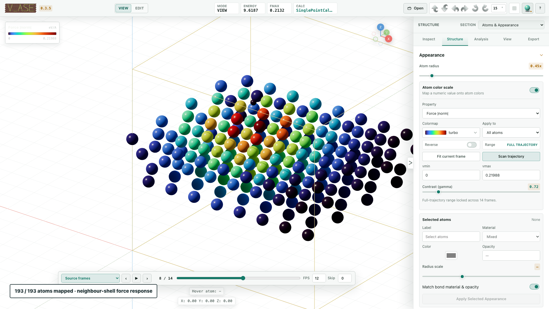
Open Structure > Appearance > Color scale. Enable it, then select a field, map, scope, range, and contrast.

Available fields are discovered lazily. Built-ins include:

• position:x, position:y, position:z;

• force:norm when stored forces exist;

• numeric per-atom ASE arrays;

• stored per-atom calculator results; and

• finite numeric LAMMPS atom columns such as custom c_* or f_* fields.

Multidimensional arrays expose norms and suitable individual components. Do not guess model-specific names: use the field list generated for the live trajectory.

Scope

• All atoms maps every visible atom with a finite value.

• Selected atoms only maps the current GUI selection. Semantic callers can pass explicit indices with scope:"selected" to freeze a stable subset independently of later human selection changes; omit indices only when the colorscale should intentionally follow the live selection.

A partially colored all-atom frame is not a successful application. Missing or nonfinite values must remain explicitly unavailable.

Range modes

GUI action/API mode	Exact meaning
Fit current frame / current	Resolve one finite range from the active frame, then keep it locked during playback
Scan trajectory / trajectory	Resolve one global finite range over every frame and reuse it
Manual vmin/vmax / manual	Use an explicit finite range with vmax > vmin

Never normalize each frame independently when comparing a trajectory. A global scan uses a bounded cached scalar buffer when possible; larger inputs remain backend-side for extrema scanning.

Colormaps and gamma

Preset maps come from the installed Matplotlib registry and include complete 0–1 preview samples. Reverse changes direction. Gamma is valid from 0.1 to 5.0; 1.0 is neutral.

Custom maps contain 2–64 unique positioned #RRGGBB stops and use continuous interpolation or discrete bands. Their definition persists in visual settings, projects, HTML, and exports. Disabling the colorscale immediately restores the saved label/element appearance and stops per-frame colorscale work.

Radial and finite pair distributions

See the dedicated RDF guide for equations, finite-size effects, cutoff boundaries, and a complete Python-to-CSV example.

Open Analysis > Radial / Pair Distribution. v_ase selects the scientifically defined quantity from boundary conditions:

Fully periodic 3D structures

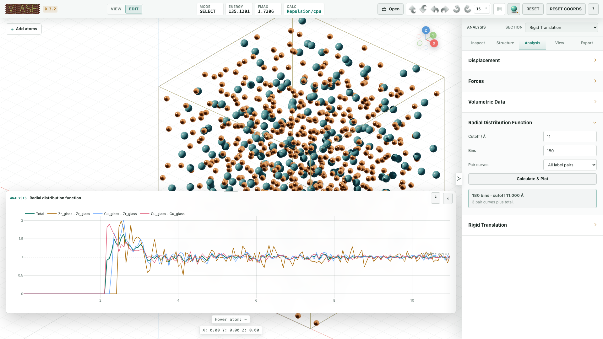
With all three periodic axes and a finite cell, v_ase computes bulk radial distribution g(r) with exact spherical-shell normalization. The requested cutoff may exceed the unique minimum-image radius. The backend enumerates all periodic images inside the requested sphere and reports the actual image extent/span; it is not limited to a fixed 2 x 2 x 2 display supercell.

The Plotly graph includes a dotted g(r) = 1 bulk reference. A sufficiently large independent random periodic model approaches that reference in an ensemble average. A finite sample has fluctuations and the conventional normalization has a finite-N exclusion effect; homogeneous placement is a correlated initialization, not an ideal-gas reference.

Finite nonperiodic structures

With no periodic axes, v_ase computes the probability density of unordered pair distances in Å⁻¹. It does not invent a bulk number density. When the cutoff contains every pair, the total curve integrates to one.

Partial periodicity

Slab and wire cells with partial PBC are rejected because a geometry-specific boundary correction is required. v_ase does not report a boundary-biased curve under the bulk RDF name.

Pair curves

Choose:

• Active bond pairs for enabled label pairs from the bonding definition;

• Selected active bond pairs for active pairs whose endpoints are both selected;

• All label pairs; or

• Total only.

The total curve is always present. Selected mode changes only the pair filter; partial curves retain full-structure normalization. Labels are exact complete user-facing identifiers.

Set a cutoff and 8–5000 bins, then choose Calculate & Plot. The graph follows the displayed source/optimizer frame and committed coordinate edits. Its save action exports the plotted total and partial columns as CSV.

Analysis frame synchronization

Changing a displayed frame refreshes every enabled frame-dependent result:

• RDF or finite pair distribution;

• atom colorscale values;

• stored force vectors;

• displacement vectors; and

• frame-associated volumetric surfaces and planes.

Ordinary-sized RDF frame/results are prefetched for smooth playback; larger products use a bounded rolling window. A pending result may leave the previous curve visible until calculation completes, but semantic verification must confirm the reported result frame. A missing frame-associated volumetric field is hidden rather than reusing stale data.

Rigid-translation timeline

Analysis > Rigid Translation can activate a selected component in either:

• two-coordinate In-plane (hkl) mode; or

• bounded 3D Cartesian mode.

Manual G or optimizer steps translate every selected atom equally, preserve all internal selected vectors, leave host atoms and cell unchanged, and use a separate registry timeline. Apply & Exit commits one Undo entry; Cancel restores the exact mode-entry coordinates. See Periodic interfaces for registry maps and calculator semantics.

Export a trajectory video

Image, video, and HTML use the shared persistent Render Area. Verify its crop, camera, frame overlays, background, axes, and cell before encoding. Video supports H.264 MOV and MPEG-4 AVI, 1–60 FPS, and optional interpolation.

For N source frames and interpolation multiplier m, the encoded count is:

(N - 1) m + 1

At 1x, every source frame appears exactly once. Minimum-image interpolation can follow periodic crossings when stable atom count, order, elements, and labels permit it. Visible displacement/force vectors and scalar colors are recomputed for each captured frame.

Semantic examples

Select a frame and refresh displacement vectors:

{
  "expectedRevision": 12,
  "frame": 12,
  "operation": {
    "name": "refresh-displacements",
    "display": {
      "showDisplacements": true,
      "displacementReferenceMode": "frame",
      "displacementReferenceFrame": 0,
      "displacementMic": true,
      "displacementStyle": "3d",
      "displacementScale": 1.0,
      "displacementThickness": 0.08,
      "displacementColor": "#e58b2a"
    }
  }
}

Enable trajectory-global colors and stored forces:

{
  "expectedRevision": 13,
  "display": {
    "showForceVectors": true,
    "forceVectorStyle": "3d",
    "forceVectorScale": 2.5,
    "forceVectorThickness": 0.10,
    "forceVectorColor": "#c43f5e"
  },
  "operation": {
    "name": "set-atom-colorscale",
    "enabled": true,
    "field": "force:norm",
    "map": "viridis",
    "scope": "all",
    "rangeMode": "trajectory",
    "gamma": 1.0
  }
}

Calculate and export RDF data:

v_ase api "$COMMAND_URL" apply --params '{
  "expectedRevision":14,
  "operation":{"name":"calculate-rdf","cutoff":6.0,"bins":300,"pairMode":"all"}
}'
v_ase api "$COMMAND_URL" export --save rdf.csv --params '{
  "format":"rdf-csv","cutoff":6.0,"bins":300,"pairMode":"all"
}'

For automation, use describe().analysis.frameSynchronization to verify that the displayed frame, RDF, colors, forces, displacements, and volumetric data all identify the same frame.

Rapidly visiting another frame and returning also refreshes invalidated field meshes. A hidden isosurface or plane is not treated as a completed cached render. The example revisions are illustrative. Re-run describe after each mutation and use its current collaboration.revision.

Verification checklist

• confirm source and active timeline kind;

• verify frame count, active frame, atom identity, and selection mapping;

• verify displacement reference and MIC policy;

• prove stored forces exist without calculator evaluation;

• record scalar field ID, scope, map, gamma, and one locked range;

• distinguish periodic RDF from finite pair density and reject partial PBC;

• verify result frame, cutoff, bins, normalization, pair curves, and warnings;

• decode video frame count and duration; and

• never accept a stale frame-specific buffer because its colors or shape look plausible.

Deterministic video frames

MOV and AVI exports encode one indexed raster per source or interpolated frame. Frame timestamps come from the chosen FPS, not the time taken to render. With N source frames and interpolation factor k, the output contains (N−1)k+1 frames, including both endpoints. Native dimensions must be even integers in 64..8192; FPS is 1..60, and interpolation is an integer from 1 through 64. The GUI retains its 256-pixel minimum input controls. Encoding never pads a typed request or invents a missing scientific frame. PNG uploads apply encoder backpressure so only one raster needs to be staged at a time. Video is opaque.

The original GUI frame is restored after export. Semantic edits and another capture wait until the video is complete. Closing the page aborts its encoder; failed sequences do not return a partial movie as a successful export.